In this tutorial, I will show you step-by-step how to perform a chi-square test of independence by using Microsoft Excel.
Example data
Let’s say I have a sample of 200 people that visited my local pub. From these 200 participants, half were male and half were female.
I asked each participant if they were a smoker or non-smoker. Here are my results:
| Smokers | Non-smokers | |
|---|---|---|
| Male | 29 | 71 |
| Female | 16 | 84 |
So, there were 29 males that smoked, and 71 that didn’t. For the females, there were 16 smokers and 84 non-smokers. Since these are the actual values from my experiment, they are known as the observed values.
What I want to do is to perform a chi-square test of independence to see if there is an association between gender and smoking status in my sample.
How to perform a chi-square test of independence in Excel
In the first part of this tutorial, I will show you how to manually perform the chi-square test in Excel, including calculating the chi-square statistic and p-value.
In the latter part of the tutorial, I will describe how to use an Excel function (CHISQ.TEST) to calculate the p-value quickly from the observed and expected values.
1. Calculate the row, column and overall totals
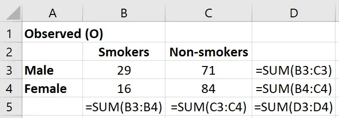
The first step to performing a chi-square test is to add up each of the rows and columns in the contingency table by using the SUM function.
=SUM(number1, [number2], ...)
So, to calculate the total in the smokers column, I will use the following formula in a new cell.
=SUM(B3:B4)
So, in total, there were 45 smokers.
I now need to repeat this process for the next column, as well as the rows in my table. Additionally, you need to calculate the overall total from your table.
The image below shows all of the formulas used for my example.
2. Calculate the expected values
Moving on, you next need to work out the expected value for each entry in the table.
To work out the expected value, you must multiply each row total by each column total, and divide that answer by the overall total.
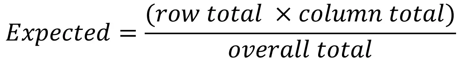
To work out the expected number of male smokers in my example, I will use the following formula.
=(D3*B5)/D5
So, in my example, the expected number of male smokers was 22.5.
Again, this process needs to be repeated for all entries in the contingency table.
3. Calculate the difference between the observed and expected values
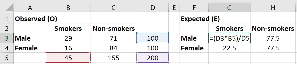
The next step is to subtract each of the expected from the observed values, square it, then divide that answer by the expected value.
So, for my example, I will use the following formula for the male smokers.
=(B3-G3)^2/G3
This process needs to be repeated for the rest of the entries in the table.
4. Calculate the chi-square statistic
Next, we need to calculate the chi-square statistic.
To do this, simply add up all the values that were recently calculated in step 3.
For my example, I will use the following formula.
=SUM(K3:L4)
So, the chi-square statistic for my example was 4.85, when rounded.
5. Calculate the degrees of freedom
Next, we need to calculate the degrees of freedom.
Here, the degrees of freedom is calculated by firstly subtracting 1 from the number of rows in the test, and multiply this answer by the number of columns in the test subtract 1.

So, for my example, I have 2 rows and 2 columns. This means to work out my degrees of freedom, I use the following calculation (you can just perform this manually, as it’s very simple math).
(2-1) x (2-1)
Which gives an answer of 1. So, this example has a degrees of freedom of 1.
6. Calculate the p-value
The final step in performing the chi-square test is to take the chi-square statistic and degrees of freedom values, and work out the p-value.
To do this in Excel, you can use the CHISQ.DIST.RT function.
=CHISQ.DIST.RT(x, deg_freedom)
- x – The cell containing the chi-square value
- deg_freedom – The cell containing the degrees of freedom value
In my example, I get a p-value of 0.028, when rounded.
7. [Optional] Use the CHISQ.TEST function to calculate the p-value
There is a function you can use to calculate the chi-square p-value by just using the observed and expected table values.
To do this, use the CHISQ.TEST function.
=CHISQ.TEST(actual_range, expected_range)
- Actual range – The cells containing the observed values
- Expected range – The cells containing the expected values
Interpreting the results
To interpret the p-value, you need to state the my two hypotheses (null and alternative).
Here are my hypotheses for my example.
- Null hypothesis – There is no association between gender and smoking status
- Alternative hypothesis – There is an association between gender and smoking status
If my alpha level, or significance threshold, was set at 0.05, this would mean I will fail to reject the null hypothesis if p>0.05. On the other hand, if p<0.05, I will reject the null hypothesis, and accept the alternative hypothesis.
In this case, my p-value was 0.028. Since this was less than 0.05, I will reject the null hypothesis, and accept the alternative hypothesis.
Therefore, there does seem to be an association between gender and smoking status.
How to perform a chi-square test of independence in Excel: Final words
After following this guide, you should now know how to perform a chi-square test of independence by using Microsoft Excel.
The steps described will calculate the chi-square statistic, degrees of freedom and the p-value. Alternatively, for a quick and easy way of generating a p-value, simply use the CHISQ.TEST function.
Microsoft Excel version used: 365 ProPlus

")
