In this step-by-step tutorial, I’m going to show you how to calculate a weighted average in Microsoft Excel. Specifically, I will demonstrate calculating a weighted average with percentages.
What is a weighted average?
The standard arithmetic average is the sum of the data values, divided by the number of data values in the dataset. In this calculation, each data value is treated equally.
On the other hand, the weighted average is the sum of each data value multiplied by their weight, divided by the sum of the weights. In this calculation, data values with higher weights have more influence over the final average, compared with values with lower weights.
Example data
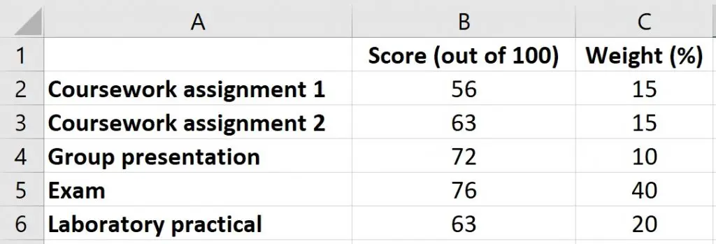
For this tutorial, let’s say I’m a teacher at a school. In my class, each student if given marks out of 100 for 5 different tests:
- Coursework assignment 1
- Coursework assignment 2
- Group presentation
- Exam
- Laboratory practical
The scores displayed in this example are just for one student. So, this particular student scored 76 out of 100, or 76% on the exam.
Each test is given a different weight. Specifically, each coursework assignment are given weights of 15%, the group presentation 10%, the exam 40% and the laboratory practical 20%.
How to calculate a weighted average in Excel
I’ll now show you two methods to calculate the weighted average in Excel. The first method is slightly long, but I will show you as it helps to understand the formulas involved. The second method uses the SUMPRODUCT function to quickly calculate the weighted average.
Method 1: Manually calculating the weighted average
Step 1: Multiply each score by the weight
To calculate the weighted average, you firstly have to multiple each score by its weight.
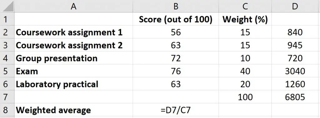
For example, for the coursework assignment 1, I will multiply 56 by 15. This is then repeated for all the tests.
The image below shows the formulas used for my example.
Step 2: Add up all the values from step 1
Next, simply add up all the values calculated from step 1.
You can easily do this by using Excel’s SUM function.
=SUM(number1, [number2], ...)
Remember to add in the desired cell range within the brackets.
So, for my example, the formula will be =SUM(D2:D6). Doing so gives a value of 6805.
Step 3: Add up the weights
Again, by using the SUM function, add up all the weights.
For my example, I will use the formula =SUM(C2:C6).
I get a value of 100.
Step 4: Divide the answer from step 2 by the answer from step 3
Finally, to calculate the weighted average, you need to divide the value from step 2 by the sum of all weights (answer from step 3).
Doing this for my example means I divide 6805 by 100, which comes to 68.05.
Since my score is out of 100, I can say that this student had a weighted average of 68.05%.
Method 2: Use the SUMPRODUCT to calculate the weighted average
This first method I have just demonstrated is a slightly long-winded approach. I purposely did this to demonstrate how to calculate the weighted average manually.
I’ll now show you how to do this quickly, by taking advantage of Excel’s SUMPRODUCT and SUM functions.
The SUMPRODUCT essentially performs steps 1 and 2 from the first method described above.
In a new cell, simply use the following formula.
=SUMPRODUCT(array1, [array2], [array3], ...)/SUM(number1, [number2], ...)
- SUMPRODUCT – Within the brackets, replace array1 with the range of cells containing the score, and replace array2 with the range of cells containing the weights
- SUM – Within the brackets, insert the range of cells containing the range of cells containing the weights
For my example, the formula will be =SUMPRODUCT(B2:B6,C2:C6)/SUM(C2:C6).
Weighted average in Excel: Final words
Now you know how to calculate the weighted average by using Microsoft Excel.
The first method describes the step-by-step approach to calculating the weighted average.
The second method uses the SUMPRODUCT and SUM functions to calculate the weighted average in a single step.
Microsoft Excel version used: 365 ProPlus


