In this tutorial, I will show you how to use the Data Analysis ToolPak to return some descriptive statistics about your data in Microsoft Excel. This includes the mean, standard error, median, mode and so much more.
How to install the Data Analysis ToolPak
A useful feature in Excel that many people do not know about is the Data Analysis ToolPak.
The Data Analysis ToolPak is an add-on created by Microsoft to make it easier to perform different data analysis procedures.
To ensure you have the Data Analysis ToolPak activated correctly, go to File>Options.
Then select Add-ins.
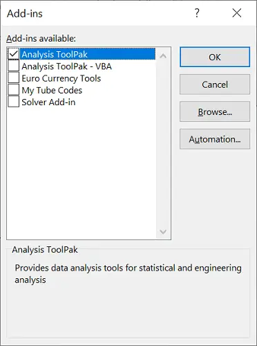
At the bottom, where it says Manage, ensure you select Excel Add-ins and click Go.
Ensure you have the Analysis ToolPak option ticked, and click the OK button.
Now, when you select the Data tab at the top, you should see a Data Analysis button appears.
Now we’re ready to perform the descriptive statistics.
How to perform descriptive statistics in Excel
To perform descriptive statistics in Excel, go to Data>Data Analysis.
Then, from the list, select Descriptive Statistics.
This should open a new window.
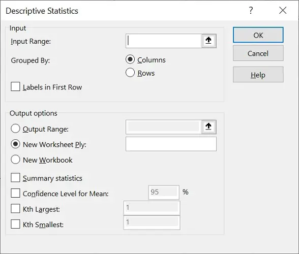
For the input range, this is where you enter the range of cells containing your data.
Next, need to tell Excel how your data are entered in your sheet.
If you have the values stacked in a column, then these will be grouped by columns. If they were entered into rows instead, then select the rows option.
If you also have labels at the top of your data in the first row, then ensure you select Labels in First Row.
For the output options, this is where you specify where you want the descriptive statistics to be returned
There are three options:
- Output Range – Enter a specific cell in this same worksheet where you want the results to be entered
- New Worksheet Ply – Enter the results in a new worksheet
- New Workbook – Enter the descriptive statistics in an entirely new Excel file
Underneath, you can tick the various descriptive statistic options that you want to perform. At a minimum, you will want to select the Summary Statistics. The Confidence Level for Mean, Kth Largest and Kth Smallest options are optional, and I will explain more about these later.
So that’s the setup done, now press the OK button to perform the descriptive statistics.
How to interpret the descriptive statistics results
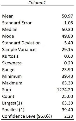
Below are some descriptive statistics I have based on some example data. I’ll now go over and explain each output.
Mean
The first result is the mean, or average, value.
This is where you add all the values up in your sample and divide by the number of values in the sample.
To calculate the mean value youself, you can use the AVERAGE function.
=AVERAGE(data)
Standard error
The standard error is a measure of the variability of sample means in a sampling distribution of means.
The higher the standard error, the higher the variability.
You can calculate the standard error yourself by taking the standard deviation and dividing it by the square root of the count.
=STDEV.S(data)/SQRT(COUNT(data))
Median
Say we sorted our data in ascending order from smallest to largest. The median will be the number that lies in the middle of the values, in my case, the answer is 50.3.
You can calculate the median separately by using the MEDIAN function.
=MEDIAN(data)
Mode
The mode represents the value that appears the most in the sample
The mode for my example is 49.8 since this value appears twice.
If you want to calculate this yourself, you can use the MODE.SNGL function.
=MODE.SNGL(data)
Standard deviation
The standard deviation is a measure of the amount of variation in the data relative to the mean, where the higher the standard deviation, the higher the variability.
If you would like to calculate the standard deviation of a sample separately from the descriptive statistics, then use the STDEV.S function.
=STDEV.S(data)
Variance
The variance is simply the square of the standard deviation.
The Excel function for the variance of a sample is VAR.S.
=VAR.S(data)
Kurtosis
Kurtosis is a measure that defines how heavily the tails of a distribution differ from the tails of a normal distribution.
In Excel, a normal distribution has a kurtosis value of 0, positive values indicate a relatively peaked distribution and negative values indicate a relatively flat distribution.
You can use the KURT function to calculate the kurtosis separately.
=KURT(data)
Skewness
Skewness is a measure of asymmetry of the data distribution.
A value of 0 indicates a perfectly symmetrical distribution.
If the value is between -1 and 1, but isn’t 0, then the data are considered fairly skewed. If the value is outside this range, then the data are highly skewed.
The function for skewness is SKEW.
=SKEW(data)
Range
The range is simply the difference between the smallest and largest values in the data.
Minimum
The minimum is the smallest number in the data.
You can use the MIN function to work this out yourself.
=MIN(data)
Maximum
As the name suggests, the maximum is the largest number in the data.
To calculate this separately, use the MAX function.
=MAX(data)
SUM
The sum is the total calculated when you add up all the values in the data.
Use the SUM function to do this yourself.
=SUM(data)
Count
The count is the total number of values you have in your data.
Use the COUNT function to calculate the count separately.
=COUNT(data)
Kth largest
During the descriptive statistics setup, if you selected the Kth Largest option, then you’ll also have this result too.
Say you have 1 in the box next to the Kth Largest option, this would mean the first largest value in the data will be returned – in other words, the maximum.
If a 2 was used instead, then the second largest value will be returned, and so on and so forth.
Kth smallest
Similar to the above, if you selected the Kth Smallest option during the setup, then you’ll also have this result returned.
Having 1 entered during the setup will mean the first smallest value will be determined – the minimum value.
Again, changing this input to a 2 would mean the second smallest value is returned instead.
Confidence level
The last entry in the descriptive statistics table is the confidence interval value.
This is the value you can add and subtract from the mean to calculate the upper and lower confidence intervals, respectively. Specifically, these will be the 95% confidence intervals, since 95 was entered during the setup.
If you want to learn more about calculating confidence intervals in Microsoft Excel, then check out this post.
How to perform descriptive statistics in Excel: Final words
You should now know how to calculate some descriptive statistics in Excel.
Using the Data Analysis ToolPak makes this process so much easier and quicker than using separate functions.
Microsoft Excel version used: 365 ProPlus
")

