How To Create A Linear Standard Curve In Excel

In this guide I will explain how to create a linear standard curve using Microsoft Excel and how to use it to calculate unknown sample values. I will use the BCA total protein assay standards as an example.

The dataset

To create a standard curve in Microsoft Excel, two data variables are required. One set of data must be the independent variable, which is the known values (e.g. protein standard concentrations in a BCA assay), and the other is the dependent variable which refers to the measured values (e.g. the optical density readings of the samples). The independent data is plotted on the x-axis, whereas the dependent data is plotted on the y-axis, on a scatter plot.

For this example, I will use data generated from the BCA protein assay kit to estimate total protein concentrations. To create the standard curve, I have measured the absorbance of 8 standards (25, 125, 250, 500, 750, 1000, 1500 and 2000 μg/mL total protein) and a blank sample (0 μg/mL total protein) for background corrections. Here is the data:

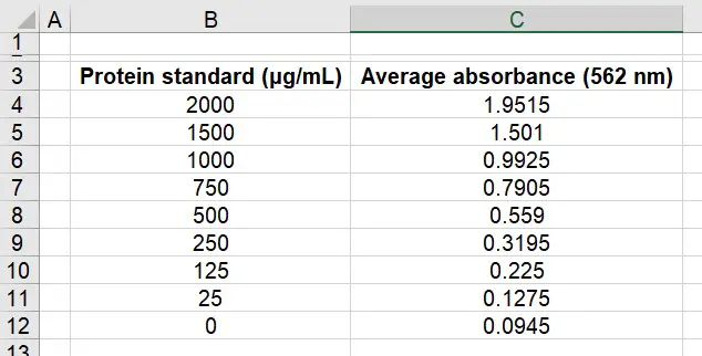What we have here is the average absorbances of each standard next to the corresponding known concentrations. In this instance, before we can proceed we need to first correct the data for the background noise.

To do this, simply subtract the average absorbance values from the average absorbance value of the blank – so ‘0.0945‘. This will give background-corrected absorbance values. I have done this below and called the column ‘Absorbance (562 nm)‘:

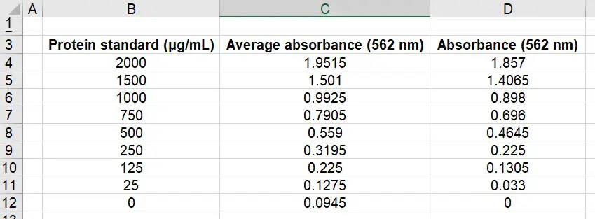You know if you have done this correctly as your corrected background sample should now read ‘0‘. See the end column in the above image.

Creating a linear standard curve in Microsoft Excel

The data is now good to create a standard curve in Excel. To do this it is easier to firstly plot a scatter plot between the known values (‘Protein standard‘) and the measured background-corrected absorbance values (‘Absorbance‘).

1. Select the two columns in Excel. To select more than one column in Excel, hold down the ‘ctrl‘ key while you click and drag the mouse over the data. Then go to, ‘Insert > Scatter‘ and select the first (‘Scatter‘) option.

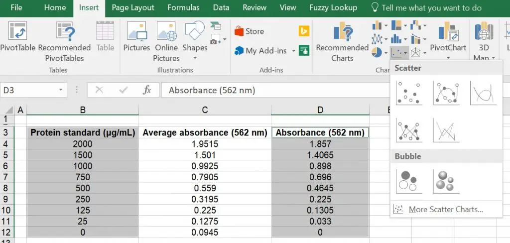2. Hopefully a scatter plot will now be displayed. We next need to create a line of best fit through each of the points in the graph to create the standard curve. For this example I will add a linear line to the graph, however, this doesn’t always have to be linear. To do this, ensure the graph is selected and go to ‘Design > Add Chart Element > Trendline > Linear‘.

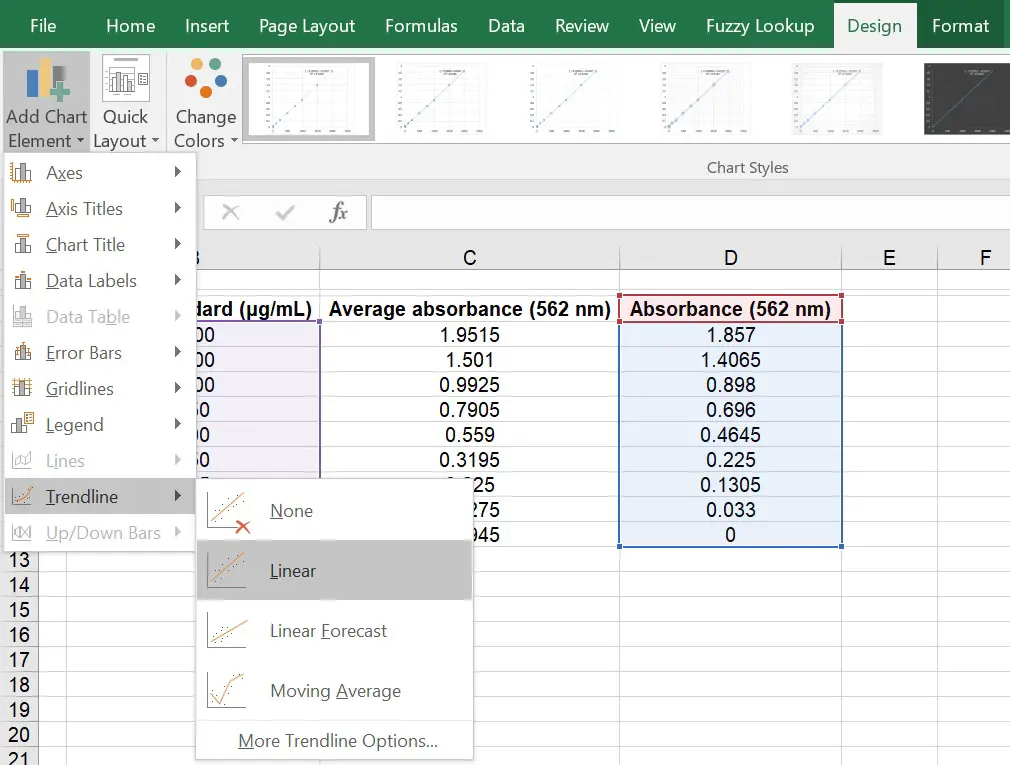Your graph should now have a linear (straight line) fit running through it. Hopefully it passes through most of your points.

3. To understand how well the linear line fits the data, it is often useful to know what the ‘R²‘ value of the line is. Simply, ‘R²‘ refers to the coefficient of determination which represents the proportion of variance for the dependent variable that is predicted by the independent variable. R² values range from 0 to 1, with 1 indicating a complete fit to the data and 0 being no goodness of fit. You may also think of the R² value as a percentage, ranging from 0% to 100%.

To display this on the graph, firstly ensure the graph is selected and go to ‘Design > Add Chart Element > Trendline > More Trendline Options …‘. A new side-menu should now appear on the right called ‘Format Trendline‘. Now, scroll down on this menu until you see the ‘Display R-squared value on chart‘ option. If you tick this, the R² value will be added onto the graph.

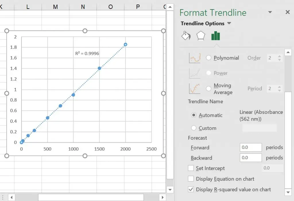You can see that the ‘R²‘ for the example is ‘0.9996‘. This indicates that the measured absorbance values are highly similar to the expected values (generated by the linear line). Alternatively, the results can be interpreted as 99.96% of the variance being explained by the linear line.

4. Additionally, the other piece of information that is required for any standard curve is the equation of the line. This can then be used to calculate the unknown samples, based on the standard curve. So, in the above example the equation can be used to work out the total protein concentrations of unknown samples.

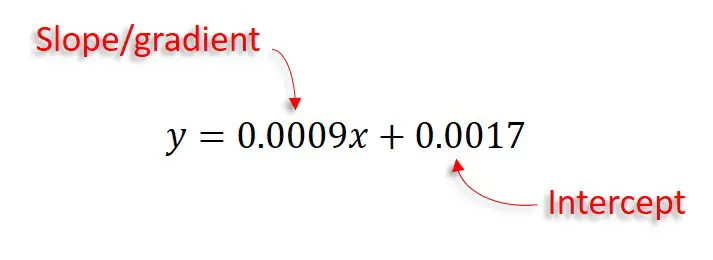
To display the equation, tick the ‘Display Equation on chart‘ option (just above the ‘Display R-squared value on chart‘) on the ‘Format Trendline‘ menu. In the above example, the equation of the line is ‘y = 0.0009x + 0.0017‘. Whereby, ‘0.0009‘ refers to the slope (gradient) of the line and ‘+ 0.0017‘ indicating the intercept of the line i.e. the point at which it crosses the y axis.

Below, I will explain how to use this equation to calculate the values for the unknown samples based on the standard curve generated.

Using the line equation to calculate unknown sample values

So you now have the equation for the line. To determine unknown values based on this, so in this example it would be using background-corrected absorbance values for unknown samples (‘y’) to work out the total protein concentration (‘x‘), you have to re-organise the equation to determine what ‘x‘ is. Let’s do this in the example:

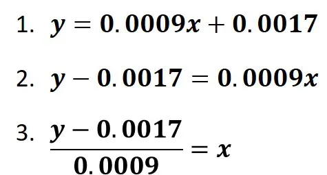Now you can just use the rearranged equation to input the ‘y‘ values in order to work out ‘x‘. For the example, let’s say we have a sample that we do not know the total protein concentration. We measure the absorbance of the sample at 562 nm and subtract the background value to account for the background signal. The sample has a background-corrected absorbance of ‘0.497‘. This would be our ‘y‘ value in the equation. Entering this would give:

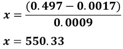So, the total protein concentration for the unknown sample is ‘550.33 μg/mL‘.

Shortcuts for calculating R² and the equation of the line

For those who want a rapid way of determining the R² and equation of the line without plotting a scatter plot, you can use the formula in Microsoft Excel to return this for you.

R²

To work out R² using an Excel formula, enter the following into a cell:

=RSQ(y values, x values)

Replace the ‘y values‘ and ‘x values‘ with your data and hit the ‘enter’ key.

Equation of the line

To work out the slope of the straight line using an Excel formula, enter the following into a cell:

=SLOPE(y values, x values)

Replace the ‘y values‘ and ‘x values‘ with your data and hit the ‘enter’ key.

To work out the intercept of the straight line using an Excel formula, enter the following into a cell:

=INTERCEPT(y values, x values)

Replace the ‘y values‘ and ‘x values‘ with your data and hit the ‘enter’ key.

Microsoft Excel version used: 2016