How To Perform A One-Sample T-Test In Excel

In this tutorial, I will show you how to perform a one-sample T-test by using Microsoft Excel.

What is a one-sample T-test?

A one-sample T-test is a statistical test to determine if a sample mean is significantly different from a hypothesized mean.

Example data

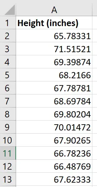
For this tutorial, I have a sample of 12 young female adults (18 years old). I measured their height in inches and entered the data into a single column in Excel.

Hypotheses

For the purpose of this example, I will pretend the national average height of 18-year-old girls is 66.5 inches.

I want to perform a one-sample T-test in Excel to determine if there is any significant difference between the heights of my sample compared with the national average height (66.5 inches).

The null and alternative hypothesis are:

• Null hypothesis – There is no significant difference between the heights of the sample, compared with the national average
• Alternative hypothesis – There is a significant difference between the heights of the sample, compared with the national average

How to perform a one-sample T-test in Excel

There is no function in Excel to perform a one-sample T-test. Instead, I will show you a step-by-step process on how to achieve this.

Firstly, calculate the mean, standard deviation (SD) and standard error of the mean (SEM) in Excel. Then, use this information to determine the t-statistic and ultimately the p-value.

Step 1: Calculate the average

The first thing you should do is to calculate the average value of the sample data.

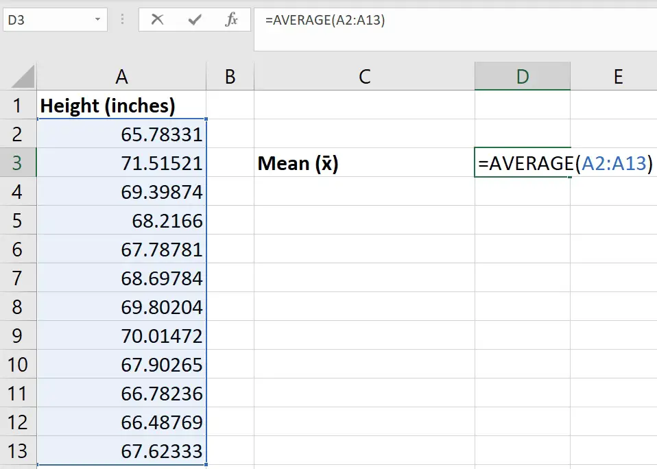
This can be easily calculated by using the AVERAGE function in Excel.

In Excel, click on an empty cell and enter the following…

=AVERAGE(cell1:cell2)

Replace cell1 in the equation with the cell containing the first data point and replace cell2 with the cell containing the last data point.

Below is a screenshot of what my example looks like.

Step 2: Calculate the standard deviation

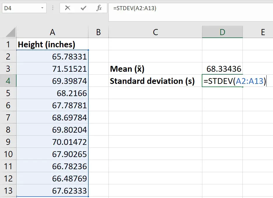
The next step is the calculate the SD of the sample data.

To do this, use the STDEV function.

In an empty cell, enter the following…

=STDEV(cell1:cell2)

Again, replace cell1 and cell 2 in the equation with the cell containing the first and last data points, respectively.

Note, you can also use the STDEV.S function to achieve the same result.

Step 3: Calculate the number of observations

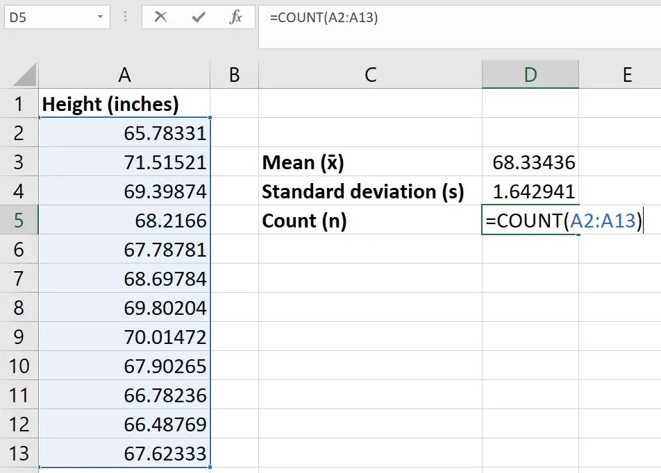
For the next step, simply count the number of observations in the sample.

This can be easily done if you have relatively small numbers. Otherwise, use the COUNT function to get Excel to count them for you.

In an empty cell, enter the following…

=COUNT(cell1:cell2)

As before, replace the cell1 and cell2 with the respected first and last cells.

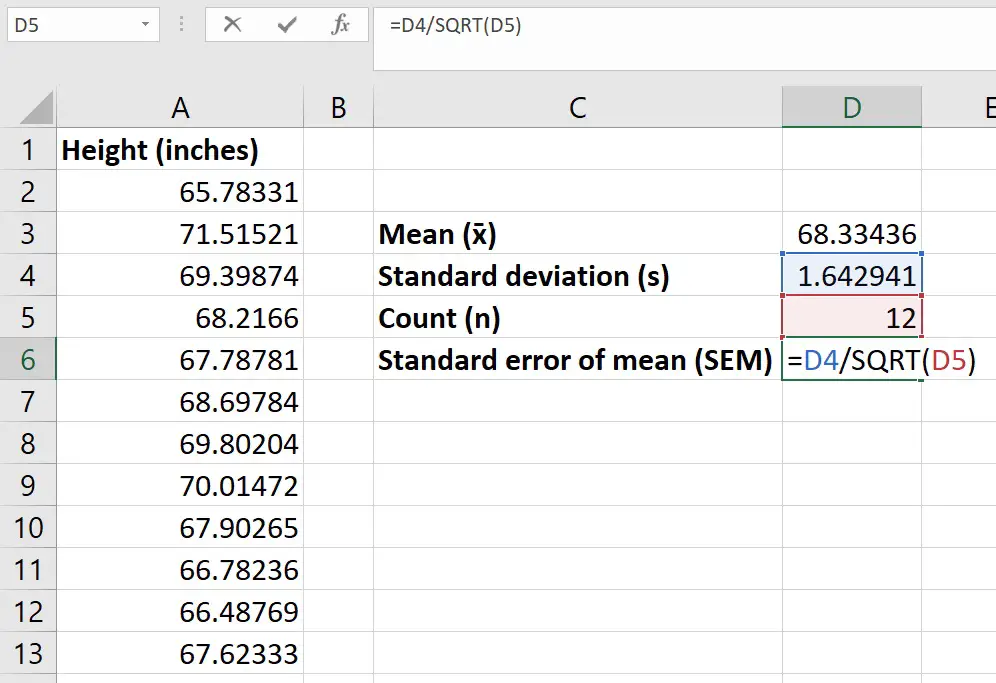
Step 4: Calculate the standard error of the mean

Now we have the mean and n, we can now work out the standard error of the mean (SEM).

To manually calculate the SEM, simply divide the SD by the square root of n.

In Excel, click on an empty cell and enter the following…

=SD/SQRT(n)

Replace the following:

• SD – With the cell containing the SD
• n – With the cell containing the n

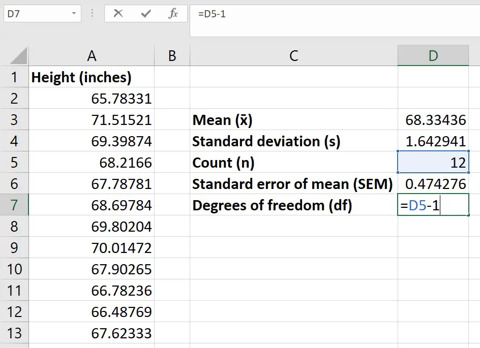
Step 5: Calculate the degrees of freedom

To calculate the degrees of freedom (df) in this case, simply subtract 1 from the n.

In a new cell, enter the following…

=n-1

Replace n with the cell containing the n.

Step 6: Calculate the t-statistic

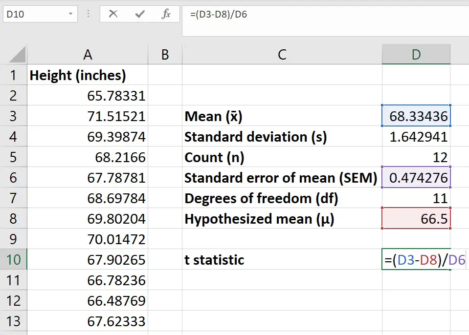
Before calculating the t-statistic, enter the hypothesized mean into a new cell in Excel.

The hypothesized mean is the value you want to compare your sample data to. So, in my example, this will be the national average height of 18-year-old girls – 66.5.

The formula to calculate the t-statistic for a one-sample T-test is shown below.

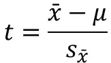
Where:

• x̄ – The sample mean
• μ – The hypothesized mean; in this case, the population mean
• s_x̄ – The SEM

So, to work this out in Excel, click on an empty cell and enter the following…

=(x̄ - μ)/sx̄  

Replace each component of the formula with the cell containing the corresponding value.

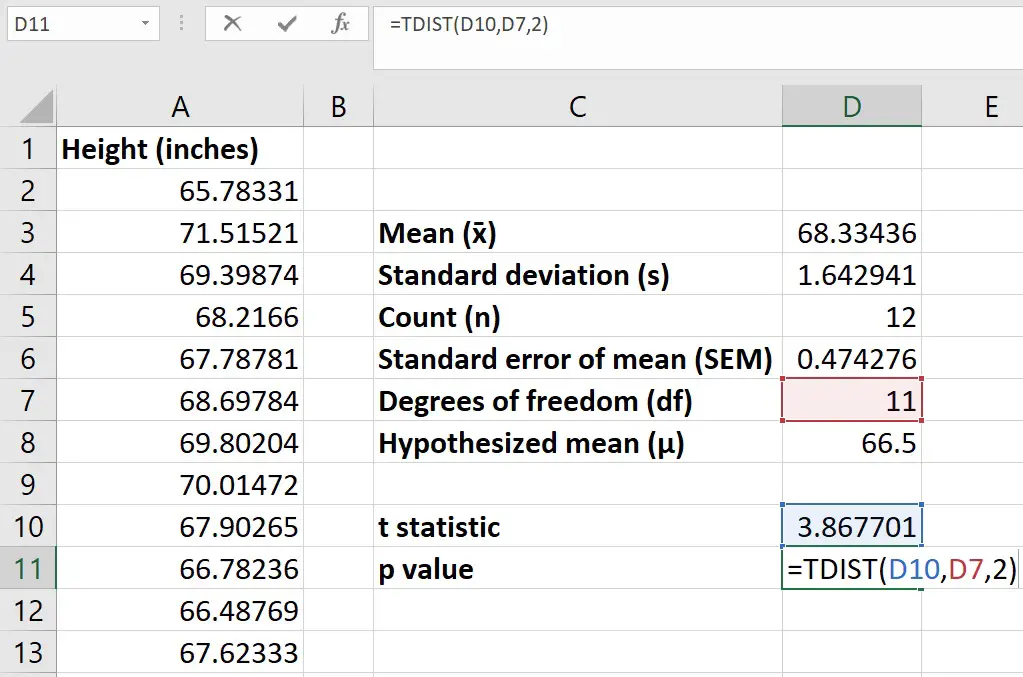
Step 7: Calculate the p-value

The last step is to calculate the p-value by using the t-statistic and the df. This is achieved by using the TDIST function.

In an empty cell, enter the following…

=TDIST(t, df, tails)

Replace the following components of the function with…

• t – The cell containing the t-statistic
• df – The cell containing the df
• tails – Enter 1 if you want to perform a one-tailed analysis, or a 2 if you want to do a two-tailed analysis

For my example, I did not hypothesize if my sample data was greater or lower than the national average. Therefore, I will perform a two-tailed analysis.

If I hypothesized the sample data will be greater than the national average, then I would select to do a one-tailed analysis instead.

So, the p-value for my example is 0.0026.

If my alpha level was set at 0.05, then since the p-value is below the alpha level, I will reject the null hypothesis and accept the alternative hypothesis.

In other words, there is a significant difference between the heights of the sample, compared with the national average.

Wrapping up

In this tutorial, I have shown you how to perform a one-sample T-test in Excel. There is no function to perform a one-sample T-test in Excel. However, you can still perform this by using a stepwise approach.

Microsoft Excel version used: 365 ProPlus