In this guide, I will show you how to perform a Spearman’s Rank correlation test in Microsoft Excel. This includes determining the Spearman correlation coefficient as well as a p value for the statistical test.
What is a Spearman correlation test?
A Spearman’s Rank correlation test is a non-parametric measure of rank correlation. It is a statistical test used to determine the strength and direction of the association between two ranked variables.
I have discussed how to perform a Pearson correlation test in Excel previously.
The output is given as the Spearman correlation coefficient (rs), which is a value ranging from -1 to 1 to indicate the strength of the association.
The following values of rs indicate the direction and strength of the association.
- rs = -1: A perfect negative association
- rs = 0: No association
- rs = +1: A perfect positive association
How to perform a Spearman correlation test in Excel
In Excel, there isn’t a function to calculate the Spearman correlation coefficient. Firstly, we need to rank the two variables to be able to calculate the correlation coefficient on the ranks.
This correlation coefficient can then be used to create a t statistic, which can then be used to determine the p value.
1. Calculate the ranks of the variables
The first step is to create two new variables, which will be the ranks. Here, I will tell Excel to rank the data in ascending order. This will assign a rank of 1 to the smallest value and so on and so forth.
To do this, we will use the RANK.AVG formula. This formula will rank the values in ascending order. Note, that if there are two values that are the same, their rank will be averaged.
In an empty column, click on the first cell and add in the following formula.
=RANK.AVG(number, ref, [order])
Replace the input requirements to…
- number: The cell containing the first data value that you want to rank
- ref: Select all of the data – this is required as a reference
- [order]: Enter a value of 1 to rank the value in ascending order
Now, repeat this process for the rest of the data points.
An easy way to do this is to lock the ref input (the range of cells containing all of the data) and dragging the formula down.
To lock the cells, add a $ symbol before the column letters and the row numbers.
Now you can safely click and drag the formula down to fill in the rest of the ranks. Since the ref cells are locked, these will remain the same.
Once you have done this, move on to the next variable and repeat the process. You should end up with two new variables containing the ranking values for the original variables.
2. Calculate the Spearman correlation coefficient in Excel
To calculate the Spearman correlation coefficient, we can use the CORREL formula with the newly created rank variables as the input.
In a new cell enter the following formula.
=CORREL(array1, array2)
Replace the input requirements to…
- array1: The range of cells for the first rank variable
- array2: The range of cells for the second rank variable
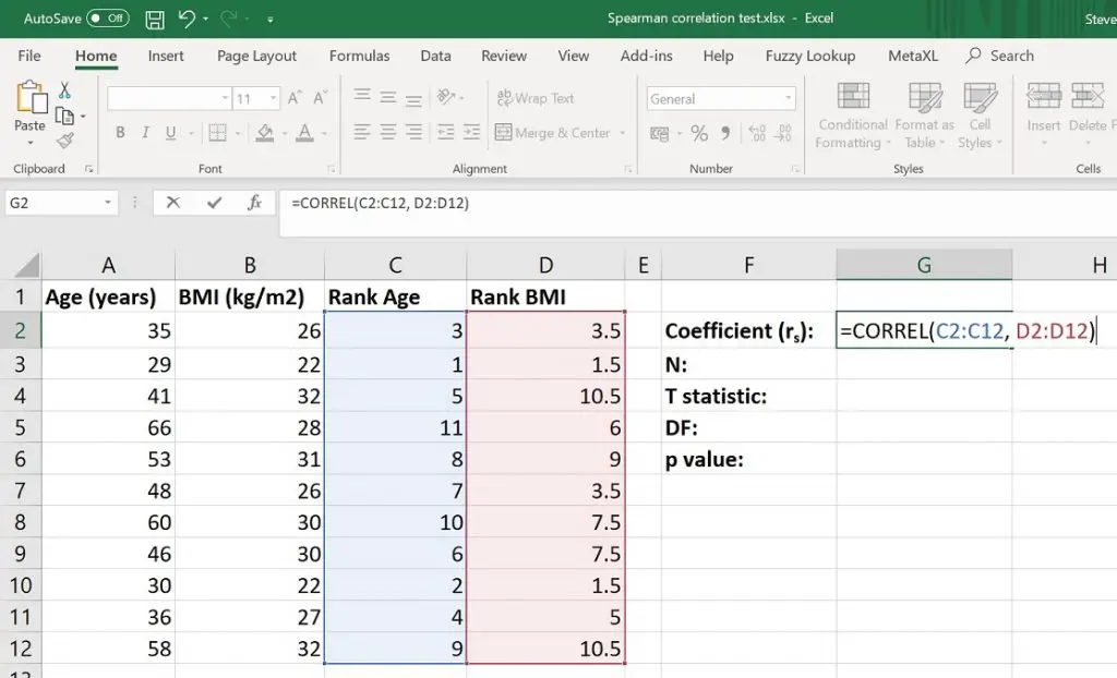
For the example above, the Spearman correlation coefficient (rs) is 0.63.
3. Calculate the number of pairs
The next step is to determine the number of pairs (n). You can just manually count them if your data is small. For large datasets, use the COUNT formula.
Note, the data should be paired. If there are missing values in one of the pairs, then you need to remove that pair from the analysis.
4. Calculate the t statistic
Next, we need to calculate the t statistic to be able to determine the p value.
There are two pieces of information we need in order to calculate the t statistic: the Spearman correlation coefficient and the number of pairs
The equation used to create the t statistic can be found below.
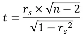
In a new cell, enter the following formula.
=(ABS(rs)*SQRT(n-2))/(SQRT(1-ABS(rs)^2))
Replace the input requirements with…
- rs: The cell containing the correlation coefficient
- n: The cell containing the number of pairs
The ABS formula is there to convert the coefficient value to an absolute value (positive number). This works when you have a negative coefficient value. Otherwise, without the ABS formula, there will be an error.
4. Calculate the degrees of freedom
Next, we need to calculate the number of degrees of freedom (DF).
The DF can be found by subtracting 2 from n.
So, in a new cell, enter the following formula.
=n-2
Replace the n with the cell containing the number of pairs.
6. Calculate the p value
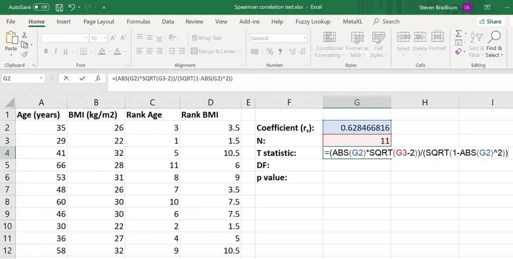
The final step is to create the p value. For this, we will use the TDIST formula.
In an empty cell, enter the following formula.
=TDIST(x, deg_freedom, tails)
Change the input to…
- x: The cell containing the t statistic value
- deg_freedom: The cell containing the DF
- tails: Enter 1 for a one-tailed analysis, or 2 for a two-tailed analysis (I will use 2 in the example)
In the example, the p value is 0.04.
Therefore, there is a significant positive correlation between participant ages and their BMI (rs=0.63, p = 0.04).
Conclusion
There is no formula in Excel to perform a Spearman’s Rank correlation test. But, there is a stepwise method to do it.
Firstly, rank the variables of interest. Then proceed to use the ranks to calculate the coefficient value, t statistic and ultimately the p value.
Microsoft Excel version used: 365 ProPlus

")
