How To Perform A Pearson Correlation Test In Excel

In this guide, I will show you how to perform a Pearson correlation test in Microsoft Excel. This includes determining the Pearson correlation coefficient as well as a p value for the statistical test.

I have discussed how to perform a Spearman’s rank correlation test in Excel previously.

What is a Pearson correlation test?

A Pearson correlation is a statistical test to determine the association between two continuous variables.

The output is given as the Pearson correlation coefficient (r) which is a value ranging from -1 to 1 to indicate the strength of the association.

The following values of r indicate the direction and strength of the association.

• r = -1: A perfect negative association
• r = 0: No association
• r = +1: A perfect positive association

If you want to learn more about about the test, including the test assumptions, then check out my Pearson correlation explained article.

How to perform a Pearson correlation test in Excel

In Excel, there is a function available to calculate the Pearson correlation coefficient. However, there is no simple means of calculating a p-value for this. A way around this is to firstly calculate a t statistic which will then be used to determine the p-value.

1. Calculate the Pearson correlation coefficient in Excel

In this section, I will show you how to calculate the Pearson correlation coefficient in Excel, which is straightforward.

In Excel, click on an empty cell where you want the correlation coefficient to be entered. Then enter the following formula.

=PEARSON(array1, array2)

Simply replace ‘array1‘ with the range of cells containing the first variable and replace ‘array2‘ with the range of cells containing the second variable.

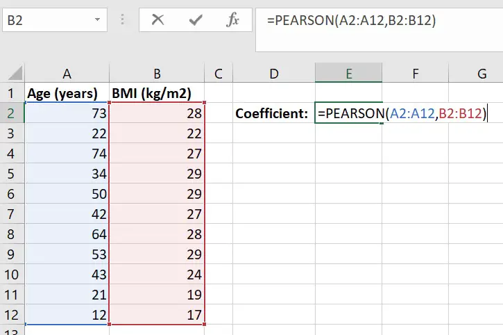
For the example above, the Pearson correlation coefficient (r) is ‘0.76‘.

2. Calculate the t-statistic from the coefficient value

The next step is to convert the Pearson correlation coefficient value to a t-statistic. To do this, two components are required: r and the number of pairs in the test (n).

In order to determine the number of pairs, simply count them manually or use the count function (=COUNT). Each pair should be a pair, so remove any entries that are not a pair.

The equation used to convert r to the t-statistic can be found below.

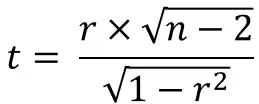
The formula to do this in Excel can be found below.

=(r*SQRT(n-2))/(SQRT(1-r^2))

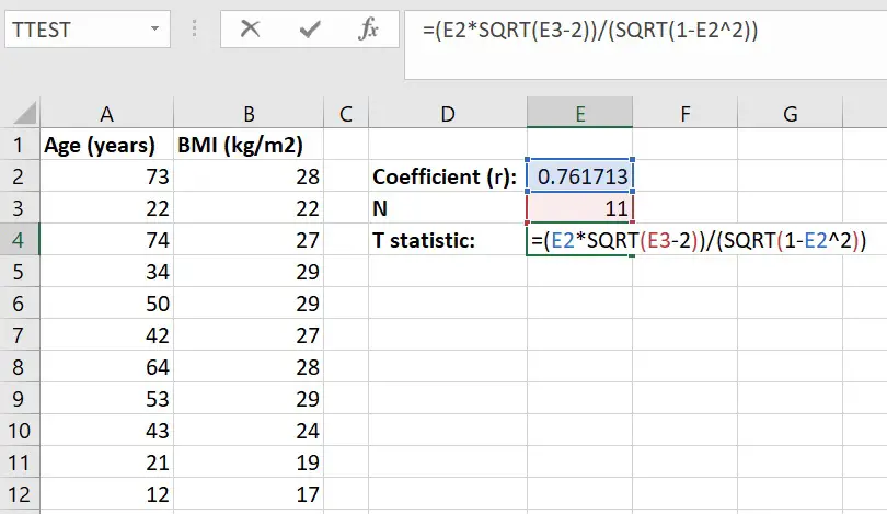
Simply replace the ‘r‘ with the correlation coefficient value and replace the ‘n‘ with the number of observations in the analysis.

For the example in this guide, the formula used in Excel can be seen below.

Note, if your coefficient value is negative, then use the following formula:

=(ABS(r)*SQRT(n-2))/(SQRT(1-ABS(r)^2))

The addition of the ABS function converts the coefficient value to an absolute (positive) number. Otherwise, a negative coefficient value will bring up an error.

3. Calculate the p-value from the t statistic

The final step in the process of calculating the p-value for a Pearson correlation test in Excel is to convert the t-statistic to a p-value.

Before this can be done, we just need to calculate a final piece of information: the number of degrees of freedom (DF). The DF can be found by subtracting 2 from n (n – 2).

Now we are ready to calculate the p-value. To do this, simply use the =TDIST function in Excel.

Simply enter the formula below.

=TDIST(x, deg_freedom, tails)

Replace the ‘x‘ with the t statistic created previously and replace the ‘deg_freedom‘ with the DF. Finally, for the tails, enter the number ‘1‘ for a one-tailed analysis or a ‘2‘ for a two-tailed analysis. If you are unsure about which to use, use a two-tailed analysis (‘2‘).

Below is a screenshot for how this looks in Excel by using the example.

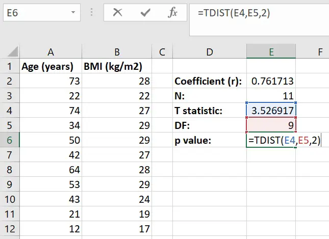
In the example, the p value is ‘0.006‘. Therefore, there is a significant positive correlation (r=0.76) between participant ages and their BMI.

Conclusion

There is no easy way to calculate a p value for a Pearson correlation test in Excel. However, by calculating the Pearson correlation coefficient this can be converted to a t-statistic, which in turn can be used to calculate a p-value.

Microsoft Excel version used: 365 ProPlus