Did you know that you can perform a t-test in Microsoft Excel? In fact, there are quite a few ways to perform a t-test in Excel. The first utilises the Data Analysis plug-in, while the second option can be used by entering a direct Excel formula. Here I will explain how to do both.
Method 1: Using the Data Analysis plug-in
Installing the Data Analysis plug-in
The first thing you need to do is make sure you have installed the Data Analysis plug-in in Microsoft Excel.
To do this, go to ‘File > Options‘. In the new window, go to ‘Add-ins‘:
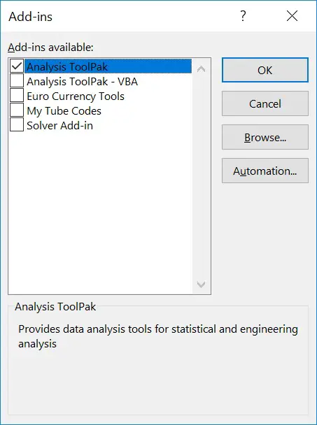
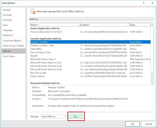 In the new window, check the ‘Analysis ToolPak‘ and click ‘OK‘.
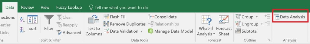
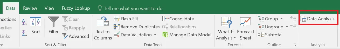
 The Data Analysis can be found under ‘Data > Data Analysis‘:
 Performing t-tests via the Data Analysis plug-in
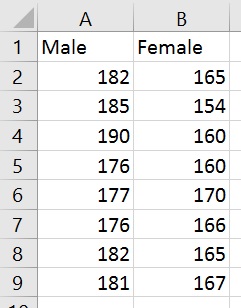
1. To perform a t-test in Microsoft Excel by using the Data Analysis plug-in, first create two columns of data. Each column should contain the values listed for each experimental group. For this guide, I will compare height (measured in cm) between a group of male and female participants.
This is how my data looks in Excel:
 2. Next, go to ‘Data > Data Analysis’.
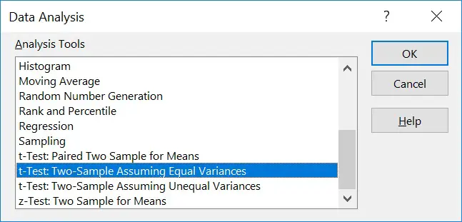 Select the t-test that is applicable to your data. There are three choices, each of which are described in more detail below.
- Paired Two Sample for Means – A paired (dependent) t-test; used when analysing data from two related groups.
- Two-Sample Assuming Equal Variances – An independent t-test; used to analyse data from two unrelated groups when the variance of the data within the groups are equal (ie the standard deviations are roughly the same).
- Two-Sample Assuming Unequal Variances – An independent t-test; used to analyse data from two unrelated groups when the variance of the data within the groups are unequal.
If you are unsure as to whether your data has an equal variance or not, first perform an F-test within Microsoft Excel.
3. For this example, I will select the ‘t-Test: Two-Sample Assuming Equal Variances’. Since I am interested in comparing data between two independent groups. I will presume the variance is equal between both groups.
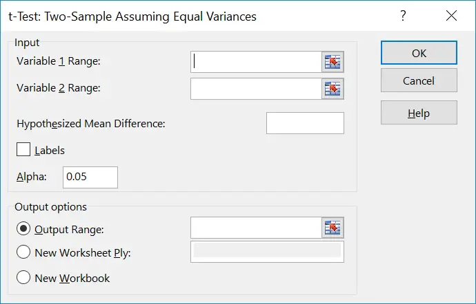
A new window will appear to allow you to select the data for each group. These are entered into the ‘Variable 1 Range’ and ‘Variable 2 Range’ sections. If your data contain headers, then tick the ‘Labels’ option.
Next, select the alpha you would like to use. The alpha is the level of significance, usually set at 0.05 (5%).
Also, select where you would like the results to be displayed. In this example, I selected ‘Output Range’ and selected an empty cell next to the data.
 The output
The output of the statistical test given is more informative than using the T-test formula directly, which only gives you the P value.
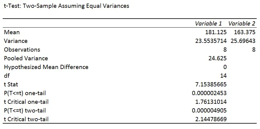
Below is an example of the output produced when using my example dataset.
 The results can be broken down into the following sections:
- Mean – The average value for each experimental group.
- Variance – The statistical variance of the data for each experimental group.
- Observations – The number of samples in each experimental group.
- Pooled variance – The average statistical variance between the two experimental groups.
- Hypothesized mean difference – If you have selected a hypothesized mean difference (which we didn’t).
- df – The degrees of freedom for the test. This is the number of values in the final calculation that may vary independently.
- t Stat – The T statistic.
- P(T<=t) one-tail – The P value, if you are using a one-tailed analysis.
- t Critical one-tail – The T statistic cut-off value when using the one-tailed analysis.
- P(T<=t) two-tail – The P value, if you are using a two-tailed analysis.
- t Critical two-tail – The T statistic cut-off value when using the two-tailed analysis.
Interpretation
In the example, the null hypothesis was:
“There is no difference in height between the males and females.”
The alternative hypothesis was:
“There is a difference in height between the males and females.”
Since I have not pre-specified which group is higher or lower than the other in the hypothesis, I will look at the output for the two-tail analysis.
By looking at this example, we can see that the P value for the two-tail analysis is ‘0.000004905‘, which is obviously less than our significance level (P<0.05). Therefore, we reject the null hypothesis and accept the alternative hypothesis.
Method 2: Using the TTEST function
There is an alternative way to perform a t-test within Microsoft Excel, by using the T-Test function. Compared to the first method, the output after using the TTEST function only produces the P value for the test.
- To perform the TTEST function, first select the cell where you want to insert the final output (the P value). Next, click ‘Formulas > Insert Function’.
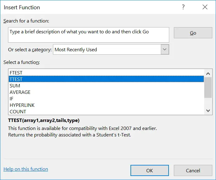 2. Scroll through the functions until you find ‘TTEST’ and click ‘OK‘. A new window will open:

Next, fill in the four required fields:
- Array1 – The data range for the first experimental group.
- Array2 – The data range for the second experimental group.
- Tails – The number of tails for the analysis
- 1 = One-tailed analysis
- 2 = Two-tailed analysis
- Type – The type of t-test to perform. Options include:
- 1 = Paired Two Sample for Means
- 2 = Two-Sample Assuming Equal Variances
- 3 = Two-Sample Assuming Unequal Variances
Press ‘OK’ to perform the test. You will now see the P value for that required test in the chosen cell.
Conclusion
In this detailed how-to guide, I have explained how to perform t-tests by using Microsoft Excel. There are two main ways to do this: through the Data Analysis plug-in or directly through the TTEST function.

")
