What is an independent t-test?

An independent t-test, also known as an unpaired t-test, is a parametric statistical test used to determine if there are any differences between two continuous variables on the same scale from two unrelated groups.

For example, comparing height differences between a sample of male and females.

The assumptions of an independent t-test

There are a few assumptions that the data has to pass before performing an independent t-test in SPSS. These are:

1. The dependent variables should be measured on a continuous scale (either interval or ratio).
2. There should be two dependent variables present which are measured from independent (non-related) groups.
3. There are no outliers present in the variables.
4. The dependent variables should be normally distributed. See how to test for normality in SPSS.
5. The dependent variables should have homogeneity of variances. In other words, their standard deviations need to be approximately the same. This can be investigated with the Levene’s Test for Equality of Variances (see below).

How to run an independent t-test in SPSS

It is always easier understanding how to do something when applying an example. So, I have done just that by using the aforementioned example for comparing height between male and females.

There are two columns in the dataset. There is a Group column which specifies if the sample is from a male or a female. In this case, 1 = males and 2 = female. This is referred to as a nominal measure, i.e. to differentiate between groups. The next column Height refers to the height (of course!) for each subject. This is classed as a scale measure, i.e. a continuous variable.

For this experiment, the null hypothesis will be:

“There is no difference in height between the males and females”.

And the alternative hypothesis will be:

“There is a difference in height between males and females”.

Performing the test

Now, let’s perform the independent t-test in SPSS.

1. First, go to Analyze > Compare Means > Independent-Samples T-Test.

2. A new window will appear. Here you need to tell SPSS which data you want to include in the independent t-test. Add the test variable (Height in this case) into the Test Variable(s): window. Also, add the grouping variable (Group in this case) to the Grouping Variable: input. The window should now look like this:

3. Next, click on the Define Groups… button. This will open up a smaller window. Here under the Use specified values header, add 1 to Group 1: and 2 to Group 2:. This is to tell SPSS that you want to compare males (Group 1) against females (Group 2). This should look like this:

4. Click the Continue button.

5. Ignore all the other buttons, such as Options and Bootstrap…, we don’t need them for this. Now click the OK button to run the test.

Output

In the output window, SPSS will now give you two boxes titled: Group Statistics and Independent Samples Test. The first box presents descriptive information about each variable (mean, number of samples and standard deviation). We only need to look at the last (Independent Samples Test) box to find the results of the independent t-test.

This is the window we need for the independent t-test interpretation. There is a wealth of numbers here which can be broken down as:

Levene’s Test for Equality of Variances

• F – The F statistic for variance testing.
• Sig. – The significance value (P value) for equal variance testing.

t-test for Equality of Means

• t – The T statistic.
• df – The degrees of freedom for the test. This is the number of values in the final calculation that may vary independently.
• Sig. (2-tailed) – The significance value (P value) for the independent t-test when applied a 2-tailed analysis.
• Mean Difference – The average difference between the two variables.
• Error Difference – The standard error for the difference between the two variables.
• 95% Confidence Interval of the Difference – The upper and lower range for the 95% confidence interval for the difference between the two variables.

Interpretation

Before you determine any statistical difference, you need to first consider if there is equality of variances between the male and female data. This can be found in the Levene’s Test for Equality of Variances section. Specifically, look at the Sig. box. If the significance value (P value) here is above 0.05, then the data does assume equal variances. Conversely, if it is below 0.05 then the data does not assume equal variances. In this example we can see that we have a Sig. of 0.776 therefore equal variances are assumed.

Now we can look to see if we have a significant result for the height difference between male and females. Under the t-test for Equality of Means section, go to the Sig. (2-tailed) column. Because we know our data assumes equal variances, we would look at the top row. Obviously, if your data does not assume equal variances then you would look at the bottom row. Our P value is 0.000 which is below our level of significance of 0.05, therefore we have a significant difference in heights between males and females.

We would reject the null hypothesis considering P<0.05 and accept the alternative hypothesis.

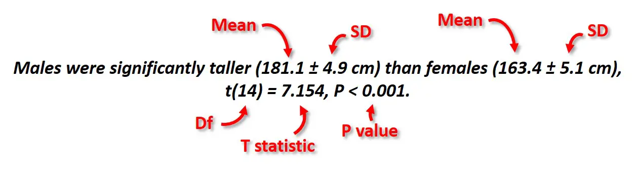
Reporting

To report the results of an independent t-test in a single sentence it is often useful to provide the mean and standard deviation for each of the variables so the reader can understand which group is significantly higher or lower than the other. Also, quoting the t statistic and degrees of freedom (Df) alongside the P value, at the end of the sentence is more informative.

The reporting of our example would read: